2010-09-06

This article describes an approach for efficient two-dimensional convolution with arbitrary circularly symmetric convolution kernels. A 2-d Gaussian kernel is linearly separable; the convolution can be split into a horizontal convolution followed by a vertical convolution. This makes 2-d Gaussian convolution relatively cheap, computationally, and “Gaussian blur” has become, partially for this reason, a popular operation in image processing. No other circularly symmetric convolution kernel is linearly separable. But this is only true when the kernel is limited to real numbers. This article introduces complex-valued convolution kernels that are both circularly symmetric and linearly separable, and goes on to show how these can be used to produce arbitrary circularly symmetric 2-d convolutions by 1-d convolutions, in contrast to the use of 2-d Fast Fourier Transform (FFT). Special focus is given to implementation of circular blur, or convolution with a solid disk, which is useful for simulation of bokeh of camera lenses with fully open apertures.

To produce circularly symmetric 2-d convolution, the condition that the 1-d kernel function must satisfy is . The condition may be broken down into a magnitude condition and a phase condition that must both be satisfied. The magnitude condition reads , meaning that the kernel must have a Gaussian function as its magnitude function. Because in multiplication of complex numbers the phases are summed, the phase (argument) condition reads , with the shorthand . The only family of functions to satisfy this is . The kernel function can be constructed as the product of a Gaussian function, here called the envelope, and a complex phasor with as its argument. In one dimension these kernels have the form , where is the imaginary unit, is the spatial coordinate, is the spatial scaling constant of the envelope, and is the spatial scaling constant of the complex phasor. In two dimensions the form is , being the coordinate in the other dimension. These forms are not normalized to preserve average intensity in image filtering, but to give a value of 1 for . Let’s see what these look like.

The real part of a phased Gaussian kernel	The imaginary part of a phased Gaussian kernel
The real part of a phased Gaussian kernel of infinite spatial scale of the magnitude part, showing the phasing only	The imaginary part of the phased Gaussian kernel of infinite spatial scale of the magnitude part, showing the phasing only	Magnitude of a phased Gaussian kernel, identical to the plain Gaussian kernel

Arbitrary circularly symmetric shapes can be constructed by a weighted sum of the real parts and imaginary parts of complex phasors of different frequencies. Fourier series is the standard approach for such designs. These give a repetitive pattern, but the repeats could be diminished by adjusting the spatial scale of the envelope. As necessary, sloping of the envelope can be compensated for in the weights of the sum, but simultaneous optimization of both will give the best results, as it can take advantage of that the envelopes need not be the same for each of the component kernels.

Let’s try a 5-component square wave approximation, designed manually with the Fourier series applet of Paul Falstad.

5-component equiripple square wave Fourier series

Real part of a square wave approximated by 5 phased Gaussian components of infinite spatial scale of the magnitude part.

The formula for this series is . A bit of scaling (by 0.9) and shifting (by -0.01) was then done to make the ripples go evenly around the zero level and to avoid values greater than 1.

This is a pretty good indicator of the capabilities of this approach. The weighted component kernels were:

Component 0

Component 1

Component 2

Component 3

Component 4

By lowering the spatial scale of the magnitude part of each component kernel, one gets a result like this:

Not so bad! The halos would need to be eliminated, and the disk is also fading a bit toward the edges.

I searched for better circular kernels by global optimization with an equiripple cost function, with the number of component kernels and the transition bandwidth as the parameters. Transition bandwidth defines how sharp the edge of the disk is. The sharper it is, the more ringing there will be both inside and outside the disk. A transition bandwidth setting of 1 means that the width of the transition is as large as the radius of the disk inside. Below, 1-d component kernel formulas are given for a pass band spanning and a dual stop band spanning .

Number of components: 1, transition bandwidth: 0.200000, ripple: ±0.232417. Component 0: (cos(x*x*1.624835) * 0.767583 + sin(x*x*1.624835) * 1.862321) * exp(-0.862325*x* x)

1-d view

Number of components: 2, transition bandwidth: 0.200000, ripple: ±0.075459. Component 0: (cos(x*x*5.268909) * 0.411259 + sin(x*x*5.268909) * -0.548794) * exp(-0.886528*x *x) Component 1: (cos(x*x*1.558213) * 0.513282 + sin(x*x*1.558213) * 4.561110) * exp(-1.960518*x* x)

1-d view of the components and their sum (magenta)

Number of components: 3, transition bandwidth: 0.200000, ripple: ±0.026297. Component 0: (cos(x*x*5.043495) * 1.621035 + sin(x*x*5.043495) * -2.105439) * exp(-2.176490*x *x) Component 1: (cos(x*x*9.027613) * -0.280860 + sin(x*x*9.027613) * -0.162882) * exp(-1.019306* x*x) Component 2: (cos(x*x*1.597273) * -0.366471 + sin(x*x*1.597273) * 10.300301) * exp(-2.815110* x*x)

1-d view of the components and their sum (cyan)

Number of components: 4, transition bandwidth: 0.200000, ripple: ±0.010843. Component 0: (cos(x*x*1.553635) * -5.767909 + sin(x*x*1.553635) * 46.164397) * exp(-4.338459* x*x) Component 1: (cos(x*x*4.693183) * 9.795391 + sin(x*x*4.693183) * -15.227561) * exp(-3.839993* x*x) Component 2: (cos(x*x*8.178137) * -3.048324 + sin(x*x*8.178137) * 0.302959) * exp(-2.791880*x *x) Component 3: (cos(x*x*12.328289) * 0.010001 + sin(x*x*12.328289) * 0.244650) * exp(-1.342190* x*x)

1-d view of the components and their sum (brown) Close-up

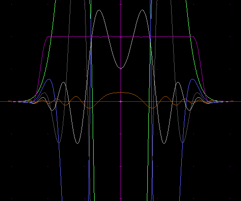
Number of components: 5, transition bandwidth: 0.200000, ripple: ±0.004062. Component 0: (cos(x*x*1.685979) * -22.356787 + sin(x*x*1.685979) * 85.912460) * exp(-4.892608 *x*x) Component 1: (cos(x*x*4.998496) * 35.918936 + sin(x*x*4.998496) * -28.875618) * exp(-4.711870 *x*x) Component 2: (cos(x*x*8.244168) * -13.212253 + sin(x*x*8.244168) * -1.578428) * exp(-4.052795 *x*x) Component 3: (cos(x*x*11.900859) * 0.507991 + sin(x*x*11.900859) * 1.816328) * exp(-2.929212* x*x) Component 4: (cos(x*x*16.116382) * 0.138051 + sin(x*x*16.116382) * -0.010000) * exp(-1.512961 *x*x)

1-d view of the components and their sum (magenta) Close-up

Close-up of the pass band Close-up of the stop band

The last one of the above, with 5 component kernels, is good enough for most practical applications as the ripple is as small as 1/250, about as much as the least significant bit for 8-bits-per-channel graphics, so invisible in almost all situations. As the number of components is increased, the components have an increasingly large weighted amplitude, as much as 36 times their sum for the 5-component system. This may become a practical problem if one aims for convolution kernel shapes with sharp transitions. A construction via Fourier series would probably give better-behaving components, but require more components than abusing the Gaussian envelope for ripple control as seems to be the case in the above given composite kernels.

Here’s a bonus, with 6 components:

The 1-d composite kernel can be truncated to range . This only necessitates a stop band equiripple condition for to ensure a flat stop band in the corners of the 2-d convolution kernel square. However, at least for up to the above given 5th order composite kernel, the stop band ripples start to slope out already within that range, so no savings can be made.

Let’s see the 5-component circular blur in action.

The standard test image, Lena
Lena after 5-component circular blur with a disk diameter of 128 pixels and an additional transition band of 25.6 + 25.6 pixels . (contrast adjusted manually)	Gaussian blur of similar size
With halved blur disk radius, 32 pixels (contrast set manually)	Gaussian blur of similar size
With 16 pixels disk radius (contrast set manually)	Gaussian blur of similar size

The circular blur here is the weighted sum of the real and imaginary parts of the 5 component convolutions. Let’s take a closer look at the first component of the 128-pixel diameter blur:

Component 0 horizontal convolution, real part (contrast is not to scale)	Component 0 horizontal convolution, imaginary part (contrast is not to scale)
Component 0 horizontal convolution followed by vertical convolution, real part (contrast is not to scale)	Component 0 horizontal convolution followed by vertical convolution, imaginary part (contrast is not to scale)

The effective convolution kernel in the last two of the above images already circularly symmetric. Let’s try another image, one which will better show the blur disks.

Hubble Deep View	Hubble Deep View after 5-component circular blur (arbitrary contrast)
With halved radius, 32 pixels (the same arbitrary contrast)	disk radius halved once more, now 16 pixels (the bands at the top and at the bottom are due to some programming bug)

Looks like an out-of-focus camera, doesn’t it?

These examples were done with 1-d finite impulse response (FIR) filters. A more efficient implementation would use 1-d FFT or pairs of 1-d causal and anti-causal infinite impulse response (IIR) filters to achieve a symmetric composite filter, if that is possible the filter coefficients being complex, I’m not sure.

The circular blur here is not perfect, because of the transition band. A completely different approach would be to calculate each blurred output pixel separately by summing the pixels that fall within the disk radius from the position of the pixel. There is a very efficient way to do this. The area of the disk can be subdivided into a minimum number of rectangular pieces and a summed area table can be used to efficiently calculate the sum of pixels within each rectangle. Here is an illustration of the idea:

To get an anti-aliased edge for the circle, the edge pixels can be summed with weights separately. Each weight will be shared by 8 edge pixels, which may give some computational savings. The complexity of this way of blurring will probably be proportional to the radius of the circle, times the logarithm of the same, perhaps. The decompositions of different size blurs could be stored in tables, which would allow also the use of a depth map to blur different parts of the image with a different disk size.

Perhaps circular blur is not the best use for the phased Gaussian kernels, as no sharp edges can be achieved. How about constructing an airy disc for low-pass filtering of the image in a manner that gives equal upper frequency limit for diagonal, horizontal and vertical features, or any direction really?